Worksheet 1

Girls in Data Science Camp

In this worksheet, we will be using a data set obtained from the Spotify Web API the top 50 tracks from 2023 (more details can be found here).

I have reduced the data set to include the following variables:

• artist_name: the artist name

• track_name: the title of the track

• album_release_date: The date when the track was released

• genres: A list of genres associated with the track’s artist(s)

• danceability: A measure from 0.0 to 1.0 indicating how suitable a track is for dancing based on a combination of musical elements

• energy: A measure from 0.0 to 1.0 representing a perceptual measure of intensity and activity

• loudness: The overall loudness of a track in decibels (dB)

• key: The key the track is in. Integers map to pitches using standard Pitch Class notation.

• tempo: The overall estimated tempo of a track in beats per minute (BPM)

• duration_ms: The length of the track in milliseconds

• time_signature: An estimated overall time signature of a track

• popularity: A score between 0 and 100, with 100 being the most popular

I also included a new variable called pop which is yes if the song falls into any type of pop genre and no otherwise.

# Load libraries

library(tidyverse)

── Attaching core tidyverse packages ───────────────────────────────────────────────────────────────── tidyverse 2.0.0 ──
✔ dplyr     1.1.4     ✔ readr     2.1.5
✔ forcats   1.0.0     ✔ stringr   1.5.1
✔ ggplot2   3.5.1     ✔ tibble    3.2.1
✔ lubridate 1.9.3     ✔ tidyr     1.3.1
✔ purrr     1.0.2     

── Conflicts ─────────────────────────────────────────────────────────────────────────────────── tidyverse_conflicts() ──
✖ dplyr::filter() masks stats::filter()
✖ dplyr::lag()    masks stats::lag()
ℹ Use the conflicted package (<http://conflicted.r-lib.org/>) to force all conflicts to become errors

# Read in the data

spotify <- read_csv("data/spotify_top_50_2023.csv")

Rows: 50 Columns: 12

── Column specification ─────────────────────────────────────────────────────────────────────────────────────────────────
Delimiter: ","
chr  (3): artist_name, track_name, genres
dbl  (8): danceability, energy, loudness, key, tempo, duration_ms, time_sign...
date (1): album_release_date

ℹ Use `spec()` to retrieve the full column specification for this data.
ℹ Specify the column types or set `show_col_types = FALSE` to quiet this message.

# Create 'pop' column 

spotify <- spotify |> 
                mutate(pop = if_else(str_detect(genres, "pop"), "yes", "no"))

head(spotify)

A tibble: 6 × 13

artist_name	track_name	album_release_date	genres	danceability	energy	loudness	key	tempo	duration_ms	time_signature	popularity	pop
<chr>	<chr>	<date>	<chr>	<dbl>	<dbl>	<dbl>	<dbl>	<dbl>	<dbl>	<dbl>	<dbl>	<chr>
Miley Cyrus	Flowers	2023-08-18	['pop']	0.706	0.691	-4.775	0	118.048	200600	4	94	yes
SZA	Kill Bill	2022-12-08	['pop', 'r&b', 'rap']	0.644	0.735	-5.747	8	88.980	153947	4	86	yes
Harry Styles	As It Was	2022-05-20	['pop']	0.520	0.731	-5.338	6	173.930	167303	4	95	yes
Jung Kook	Seven (feat. Latto) (Explicit Ver.)	2023-11-03	['k-pop']	0.790	0.831	-4.185	11	124.987	183551	4	90	yes
Eslabon Armado	Ella Baila Sola	2023-04-28	['corrido', 'corridos tumbados', 'sad sierreno', 'sierreno']	0.668	0.758	-5.176	5	147.989	165671	3	86	no
Taylor Swift	Cruel Summer	2019-08-23	['pop']	0.552	0.702	-5.707	9	169.994	178427	4	99	yes

Exercise 1: Wrangling

1.1

Is the spotify data tidy? Why or why not?

Answer: The data set is mostly tidy: each row corresponds to a single observation and each column corresponds to a single variable. However, each cell does not always correspond to a single value. For example, the genres column sometimes displays multiple genres per song (e.g., the song “Kill Bill” is clsasified as three genres: pop, r&b and rap).

1.2

What are the dimensions of this data set (i.e., the number of rows and columns)?

dim(spotify) 

1. 50
2. 13

1.3

Without examining the entire data set, which artist and track is in the 35th row of the data set? Note that your code should return only the required variables (artist_name and track_name).

spotify |> 
    slice(35) |>
    select(artist_name, track_name)

A tibble: 1 × 2

artist_name	track_name
<chr>	<chr>
Doja Cat	Paint The Town Red

1.4

Create a subset of the data that only includes tracks with a popularity score over 90. Assign this to an object called pop_90. How many songs have a popularity score over 90?

pop_90 <- spotify |> 
            filter(popularity > 90)

pop_90

A tibble: 20 × 13

artist_name	track_name	album_release_date	genres	danceability	energy	loudness	key	tempo	duration_ms	time_signature	popularity	pop
<chr>	<chr>	<date>	<chr>	<dbl>	<dbl>	<dbl>	<dbl>	<dbl>	<dbl>	<dbl>	<dbl>	<chr>
Miley Cyrus	Flowers	2023-08-18	['pop']	0.706	0.691	-4.775	0	118.048	200600	4	94	yes
Harry Styles	As It Was	2022-05-20	['pop']	0.520	0.731	-5.338	6	173.930	167303	4	95	yes
Taylor Swift	Cruel Summer	2019-08-23	['pop']	0.552	0.702	-5.707	9	169.994	178427	4	99	yes
Metro Boomin	Creepin' (with The Weeknd & 21 Savage)	2022-12-02	['rap']	0.715	0.620	-6.005	1	97.950	221520	4	91	no
Taylor Swift	Anti-Hero	2022-10-21	['pop']	0.637	0.643	-6.571	4	97.008	200690	4	92	yes
Arctic Monkeys	I Wanna Be Yours	2013-09-09	['garage rock', 'modern rock', 'permanent wave', 'rock', 'sheffield indie']	0.464	0.417	-9.345	0	67.528	183956	4	96	no
David Guetta	I'm Good (Blue)	2022-08-26	['big room', 'dance pop', 'edm', 'pop', 'pop dance']	0.561	0.965	-3.673	7	128.040	175238	4	92	yes
David Kushner	Daylight	2023-04-14	['gen z singer-songwriter', 'singer-songwriter pop']	0.508	0.430	-9.475	2	130.090	212954	4	94	yes
The Weeknd	Starboy	2016-11-25	['canadian contemporary r&b', 'canadian pop', 'pop']	0.679	0.587	-7.015	7	186.003	230453	4	95	yes
OneRepublic	I Ain't Worried	2022-05-13	['piano rock', 'pop']	0.704	0.797	-5.927	0	139.994	148486	4	92	yes
Myke Towers	LALA	2023-03-23	['reggaeton', 'trap latino', 'urbano latino']	0.708	0.737	-4.045	1	91.986	197920	4	93	no
Doja Cat	Paint The Town Red	2023-09-20	['dance pop', 'pop']	0.864	0.556	-7.683	2	99.974	230480	4	93	yes
The Neighbourhood	Sweater Weather	2013-04-19	['modern alternative rock', 'modern rock', 'pop']	0.612	0.807	-2.810	10	124.053	240400	4	93	yes
SZA	Snooze	2022-12-09	['pop', 'r&b', 'rap']	0.559	0.551	-7.231	5	143.008	201800	4	93	yes
The Weeknd	Blinding Lights	2020-03-20	['canadian contemporary r&b', 'canadian pop', 'pop']	0.514	0.730	-5.934	1	171.005	200040	4	93	yes
Jimin	Like Crazy	2023-03-24	['k-pop']	0.629	0.733	-5.445	7	120.001	212241	4	93	yes
Eminem	Mockingbird	2004-11-12	['detroit hip hop', 'hip hop', 'rap']	0.637	0.678	-3.798	0	84.039	250760	4	91	no
Olivia Rodrigo	vampire	2023-09-08	['pop']	0.511	0.532	-5.745	5	138.005	219724	4	95	yes
Tyler, The Creator	See You Again (feat. Kali Uchis)	2017-07-21	['hip hop', 'rap']	0.558	0.559	-9.222	6	78.558	180387	4	92	no
d4vd	Romantic Homicide	2022-07-20	['bedroom pop']	0.571	0.544	-10.613	6	132.052	132631	4	91	yes

nrow(pop_90) 

20

20 tracks have a popularity score over 90.

1.5

Now, I want to look at pop songs that have a danceability score over 0.7. Create a subset of the spotify data set to achieve this task, ordered from highest to lowest danceability.

spotify |>
    filter(danceability > 0.7 & pop == "yes") |> 
    arrange(by = desc(danceability))

A tibble: 13 × 13

artist_name	track_name	album_release_date	genres	danceability	energy	loudness	key	tempo	duration_ms	time_signature	popularity	pop
<chr>	<chr>	<date>	<chr>	<dbl>	<dbl>	<dbl>	<dbl>	<dbl>	<dbl>	<dbl>	<dbl>	<chr>
Ozuna	Hey Mor	2022-10-07	['puerto rican pop', 'reggaeton', 'trap latino', 'urbano latino']	0.901	0.589	-6.713	1	98.002	196600	4	87	yes
Doja Cat	Paint The Town Red	2023-09-20	['dance pop', 'pop']	0.864	0.556	-7.683	2	99.974	230480	4	93	yes
Feid	CLASSY 101	2023-03-31	['colombian pop', 'pop reggaeton', 'reggaeton', 'reggaeton colombiano', 'trap latino', 'urbano latino']	0.859	0.658	-4.790	11	100.065	195987	4	87	yes
Manuel Turizo	La Bachata	2023-03-17	['colombian pop', 'latin pop', 'reggaeton', 'reggaeton colombiano', 'trap latino', 'urbano latino']	0.835	0.679	-5.329	7	124.980	162638	4	85	yes
NewJeans	OMG	2023-01-02	['k-pop', 'k-pop girl group']	0.804	0.771	-4.067	9	126.956	212253	4	87	yes
Rema	Calm Down (with Selena Gomez)	2023-04-27	['afrobeats', 'nigerian pop']	0.799	0.802	-5.196	11	107.008	239318	4	90	yes
Jung Kook	Seven (feat. Latto) (Explicit Ver.)	2023-11-03	['k-pop']	0.790	0.831	-4.185	11	124.987	183551	4	90	yes
FIFTY FIFTY	Cupid - Twin Ver.	2023-09-22	['k-pop girl group']	0.783	0.592	-8.332	11	120.018	174253	4	75	yes
Bizarrap	Shakira: Bzrp Music Sessions, Vol. 53	2023-01-11	['argentine hip hop', 'pop venezolano', 'trap argentino', 'trap latino', 'urbano latino']	0.778	0.632	-5.600	2	122.104	218289	4	85	yes
Taylor Swift	Blank Space	2014-10-27	['pop']	0.753	0.678	-5.421	5	96.006	231827	4	78	yes
Sam Smith	Unholy (feat. Kim Petras)	2023-01-27	['pop', 'uk pop']	0.712	0.463	-7.399	2	131.199	156943	4	84	yes
Miley Cyrus	Flowers	2023-08-18	['pop']	0.706	0.691	-4.775	0	118.048	200600	4	94	yes
OneRepublic	I Ain't Worried	2022-05-13	['piano rock', 'pop']	0.704	0.797	-5.927	0	139.994	148486	4	92	yes

1.6

What is the average danceability score for Taylor Swift songs?

# Filter for only Taylor Swift songs
spotify |>
    filter(artist_name == "Taylor Swift") 

A tibble: 3 × 13

artist_name	track_name	album_release_date	genres	danceability	energy	loudness	key	tempo	duration_ms	time_signature	popularity	pop
<chr>	<chr>	<date>	<chr>	<dbl>	<dbl>	<dbl>	<dbl>	<dbl>	<dbl>	<dbl>	<dbl>	<chr>
Taylor Swift	Cruel Summer	2019-08-23	['pop']	0.552	0.702	-5.707	9	169.994	178427	4	99	yes
Taylor Swift	Anti-Hero	2022-10-21	['pop']	0.637	0.643	-6.571	4	97.008	200690	4	92	yes
Taylor Swift	Blank Space	2014-10-27	['pop']	0.753	0.678	-5.421	5	96.006	231827	4	78	yes

# Compute the average danceability score using `summarize`
spotify |>
    filter(artist_name == "Taylor Swift") |>
    summarize(avg_dance_TS = mean(danceability))

A tibble: 1 × 1

avg_dance_TS
<dbl>
0.6473333

1.7

Are Taylor Swfit’s songs more danceable than The Weekend’s? Hint: use group_by.

spotify |>
     group_by(artist_name) |>
     summarize(avg_dance = mean(danceability)) |> 
     filter(artist_name == "Taylor Swift" | artist_name == "The Weeknd")

A tibble: 2 × 2

artist_name	avg_dance
<chr>	<dbl>
Taylor Swift	0.6473333
The Weeknd	0.5885000

1.8

Are pop songs more popular than other genres? Compare the average popularity scores between pop songs vs. other genres.

spotify |>
     group_by(pop) |>
     summarize(avg_popularity = mean(popularity))

A tibble: 2 × 2

pop	avg_popularity
<chr>	<dbl>
no	87.75000
yes	88.26471

Exercise 2: Data Visualization

2.1

Using a histogram, visualize the distribution of popularity scores for Spotify’s top 50 tracks from 2023. Describe what you see.

ggplot(spotify, aes(x = popularity)) +
    geom_histogram(bins=25, fill = "cornflowerblue", color = "black") + 
    theme(text = element_text(size = 26)) + # increase text size
    labs(x='Popularity Score', y='Count', title='Popularity Score')

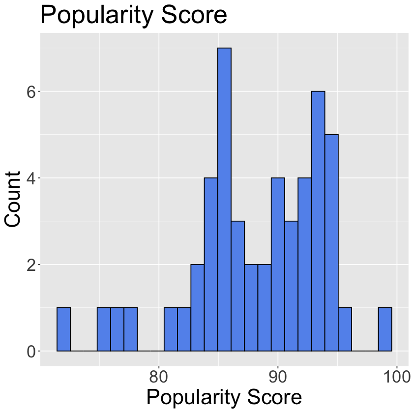
The popularity scores are distributed from about 72-99, with two main points of concentration around approximately 85 and 95.

2.2

Are pop songs more popular than other genres? You answered this in question 1.8 using summary statistics, but now use histograms to visualize the popularity groups for the two groups on the same graph. Do you notice anything different?

Hint: use facet_grid

ggplot(spotify, aes(x = popularity, fill = pop)) +
    geom_histogram(bins=25, color = "black") +
    facet_grid(rows = vars(pop)) +
    theme(text = element_text(size = 26)) +
    labs(x='Popularity Score', y='Count', title='Histogram of Popularity Score ')

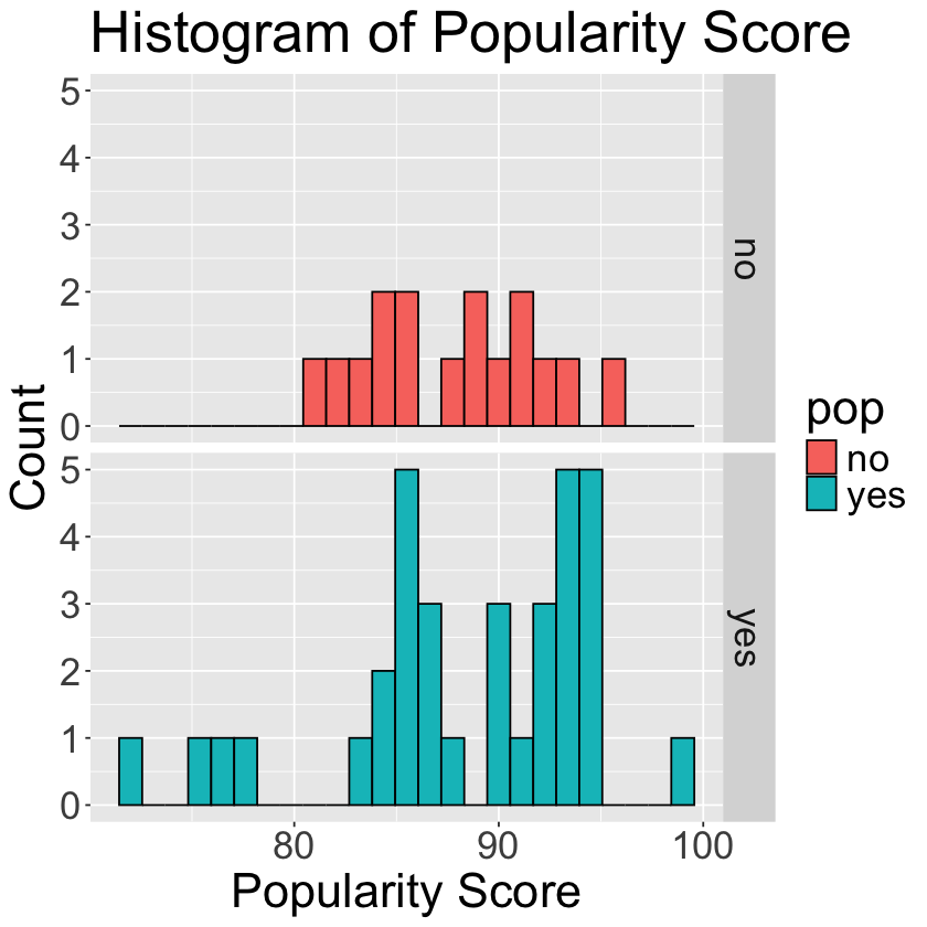
While the center of the two distributions are very similar (both around 88), we can see that the distribution of popularity scores for pop songs has more variability and a wider spread than songs that are not classified as pop.

2.3

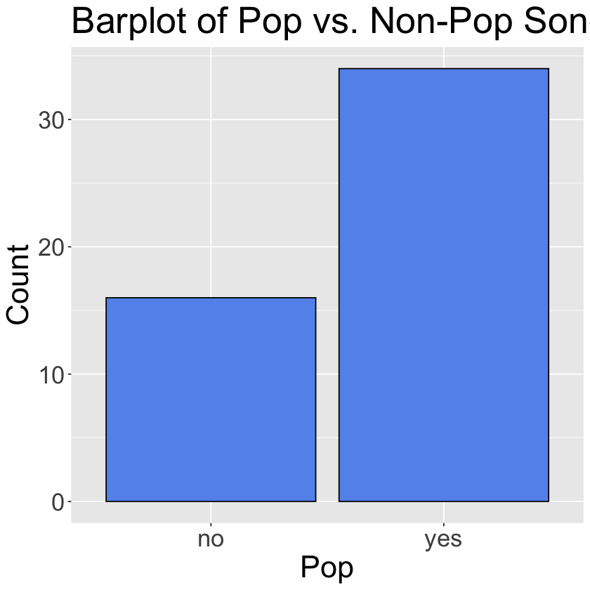
Create a barplot comparing the counts of pop songs vs. non-pop songs.

ggplot(spotify, aes(x = pop)) +
    geom_bar(fill = "cornflowerblue", color = "black") +
    theme(text = element_text(size = 26)) + 
    labs(x = 'Pop', y = 'Count', title = 'Barplot of Pop vs. Non-Pop Songs') 
  

2.4

Is there a relationship between how loud a song is in decibels and its popularity? Visualize the relationship between loudness and popularity with a scatterplot, plotting loudness on the \(y\)-axis and popularity on the \(x\)-axis. What do you notice?

options(repr.plot.width = 10, repr.plot.height = 8)

ggplot(spotify, aes(x = popularity, y = loudness)) + 
    geom_point(size=4) +
    theme(text = element_text(size = 26)) + 
    labs(x='Popularity Score', y='Loudness (dB)',title='Scatterplot of Loudness vs. Popularity') # rename axes and add title

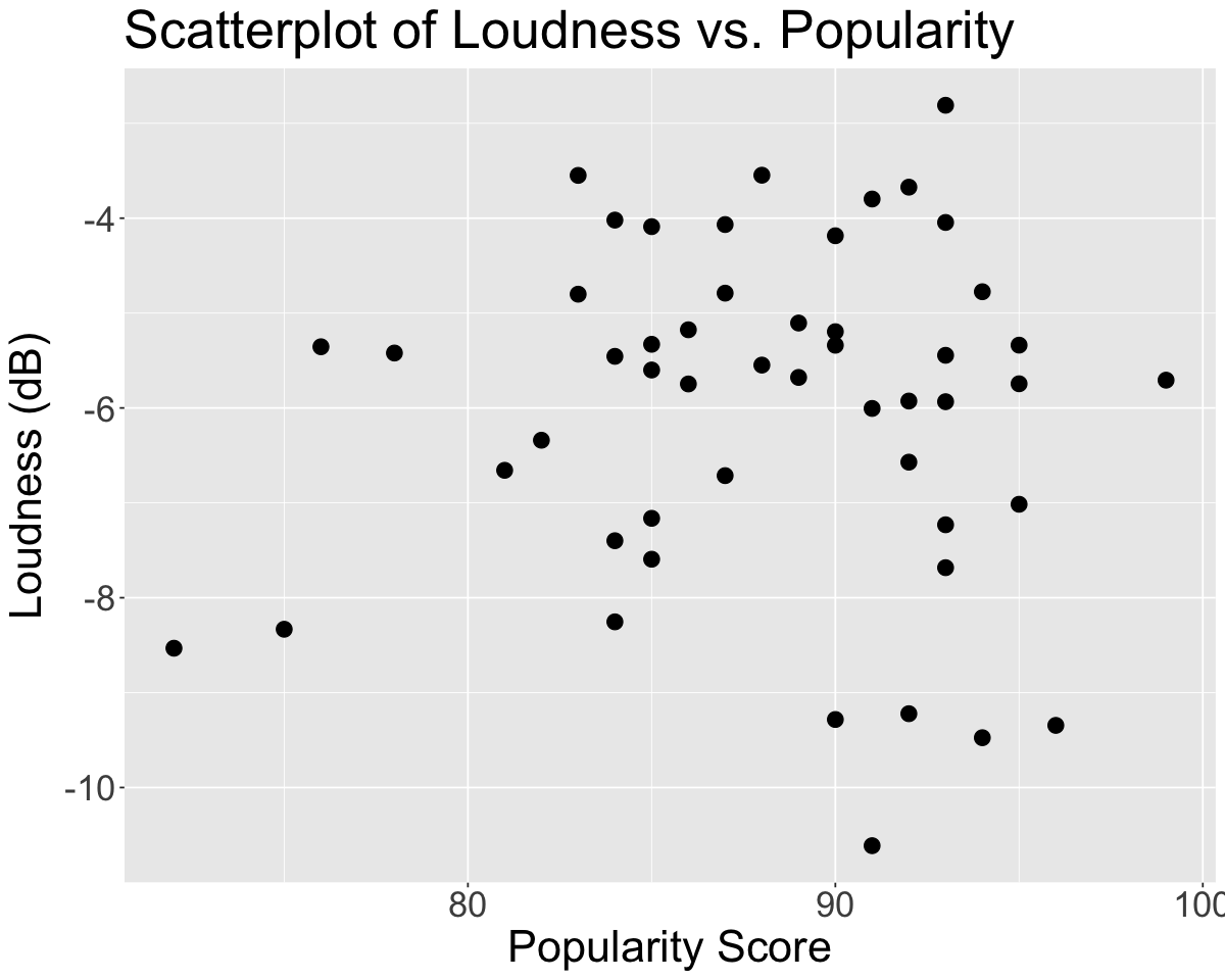
It seems like there is a relatively weak positive relationship between loudness and popularity score.

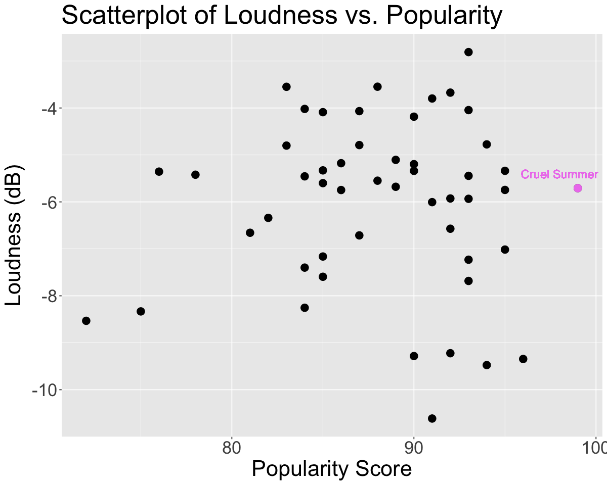
2.5 (Challenge)

Find the song that has the highest popularity score, but a relatively moderate loudness. Highlight the point on the graph and label it.

Hint: Use the annotate function to highlight a point

spotify |> 
    arrange(desc(popularity)) |>
    slice(1) |>
    select(artist_name, track_name, popularity, loudness)

A tibble: 1 × 4

artist_name	track_name	popularity	loudness
<chr>	<chr>	<dbl>	<dbl>
Taylor Swift	Cruel Summer	99	-5.707

options(repr.plot.width = 10, repr.plot.height = 8)

ggplot(spotify, aes(x = popularity, y = loudness)) + 
    geom_point(size=4) +
    annotate("point", x = 99, y = -5.707, color = 'violet', size = 4) + 
    geom_text(x = 98, y = -5.4 , label = "Cruel Summer", color = "violet", size = 5) + # add text to plot
    theme(text = element_text(size = 26)) + 
    labs(x='Popularity Score', y='Loudness (dB)',title='Scatterplot of Loudness vs. Popularity') # rename axes and add title

2.6 (Challenge)

List the artists who have more than one track in the top 50. For each artist, show the number of tracks and their average popularity score.

popular_artists <- spotify |>
    group_by(artist_name) |> 
    summarize(track_count = n(), avg_popularity = mean(popularity)) |>
    filter(track_count > 1)

popular_artists

A tibble: 6 × 3

artist_name	track_count	avg_popularity
<chr>	<int>	<dbl>
Bad Bunny	2	86.50000
Bizarrap	2	86.50000
SZA	2	89.50000
Taylor Swift	3	89.66667
The Weeknd	4	89.50000
d4vd	2	90.50000